Normal distribution

Normal

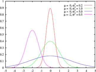
Probability density function The green line is the standard normal distribution
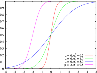
Cumulative distribution function Colors match the image above
Parameters	$\mu$ location (real) $\sigma ^{2}>0$ squared scale (real)
Support	$x\in \mathbb {R} \!$
Probability density function (pdf)	${\frac {1}{\sigma {\sqrt {2\pi }}}}\;\exp \left(-{\frac {\left(x-\mu \right)^{2}}{2\sigma ^{2}}}\right)\!$
Cumulative distribution function (cdf)	${\frac {1}{2}}\left(1+\mathrm {erf} \,{\frac {x-\mu }{\sigma {\sqrt {2}}}}\right)\!$
Mean	$\mu$
Median	$\mu$
Mode	$\mu$
Variance	$\sigma ^{2}$
Skewness	0
Excess kurtosis	0
Entropy	$\ln \left(\sigma {\sqrt {2\,\pi \,e}}\right)\!$
Moment-generating function (mgf)	$M_{X}(t)=\exp \left(\mu \,t+{\frac {\sigma ^{2}t^{2}}{2}}\right)$
Characteristic function	$\chi _{X}(t)=\exp \left(\mu \,i\,t-{\frac {\sigma ^{2}t^{2}}{2}}\right)$

For the normal distribution, the values less than one standard deviation away from the mean account for 68.27% of the set; while two standard deviations from the mean account for 95.45%; and three standard deviations account for 99.73%.

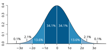
The normal distribution is a probability distribution used in probability theory and statistics. It is also called Gaussian distribution because it was first discovered by Carl Friedrich Gauss. The normal distribution is very important in many fields because many things take this form. A random variable that takes this form is normally distributed, and can be called a normal deviate. The normal distributed is often called the bell curve, because the graph of its probability density looks like a bell. The standard normal distribution (also known as the Z distribution) is a normal distribution that has a mean of zero and a standard deviation of one.

The form of the distribution is

$f(x)={\frac {1}{\sigma {\sqrt {2\pi }}}}e^{-{\frac {1}{2}}\left({\frac {x-\mu }{\sigma }}\right)^{2}}$

In a normal distribution, the parameter $\mu$ is the mean ("average"). The standard deviation ("variability") is $\sigma$. The variance of the distribution is $\sigma ^{2}$.

The normal distribution is important because it can represent real-life examples. It is used in natural and social sciences. Some examples include:

• Height
• Test scores
• Measurement errors
• Light intensity as in laser light)
• Insurance companies use normal distributions to model certain average cases.

The central limit theorem can be used to describe real-life data as a normal distribution.

Origin

Its origin goes back to the 18th century to De Moivre and in the early 19th century with Gauss.

Use

It is the most widely used piece of statistics by far. It was famously used in World War I by the United States Army to decide when men were so poor mentally that they could not be used by the Army in any job.

Related pages

• Frequency distribution
• Least squares
• Student's t-distribution

Other websites

• Cumulative Area Under the Standard Normal Curve Calculator from Daniel Soper's Free Statistics Calculators website. Computes the cumulative area under the normal curve (i.e., the cumulative probability), given a z-score.
• Interactive Standard Normal Distribution
• GNU Scientific Library – Reference Manual – The Gaussian Distribution
• Normal Distribution Table
• Download free two-way normal distribution calculator
• Download free normal distribution fitting software